
How StableSwap 2026 algorithms work
Use this section to make the StableSwap decision easier to compare in real life, not just on paper. Start with the reader's actual constraint, then separate must-have requirements from details that are merely nice to have. A practical choice should survive normal use, maintenance, timing, and budget. If a recommendation only works in an ideal situation, call that out plainly and give the reader a fallback path.
The simplest way to use this section is to write down the must-have criteria first, then compare each option against those criteria before weighing nice-to-have features.
Capital Efficiency and Slippage Comparison
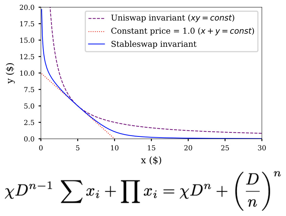
The primary distinction between StableSwap and traditional Automated Market Makers (AMMs) lies in how they handle liquidity depth for assets with correlated values. Traditional models, such as Uniswap V2, rely on a constant product formula ($x \times y = k$) that imposes severe slippage penalties on stablecoin pairs, even when price variance is minimal. StableSwap, as detailed in the Curve documentation, utilizes a hybrid invariant that behaves like a constant product for large deviations but mimics a constant sum for small deviations, thereby preserving capital efficiency where it matters most.
This architectural difference directly impacts the cost of trading for institutional and high-volume participants. In a standard Uniswap V2 pool, swapping $1 million worth of USDC for USDT can result in significant price impact due to the fixed liquidity depth. Conversely, StableSwap pools concentrate liquidity near the peg, reducing the slippage curve’s steepness. This allows for larger trade sizes without materially affecting the asset’s price, a critical requirement for stablecoin arbitrage and treasury management.
The following comparison highlights the operational metrics that differentiate these models. Note that specific slippage percentages vary based on real-time pool depth and trading volume, but the relative efficiency gap remains consistent.
For entities managing stablecoin liquidity, the choice of protocol is not merely a matter of preference but of risk mitigation. Traditional AMMs expose capital to unnecessary slippage costs, effectively acting as a tax on stability. StableSwap’s design, which prioritizes minimal price impact for correlated assets, offers a more robust framework for maintaining treasury integrity. As noted in analyses of PancakeSwap’s implementation of StableSwap, this efficiency translates to lower fees and higher yields for liquidity providers, reinforcing the model’s dominance in the stablecoin sector.
How StableSwap Mitigates Impermanent Loss
Impermanent loss arises when the price ratio of two assets in a liquidity pool diverges from the ratio at the time of deposit. In traditional Automated Market Makers (AMMs) like Uniswap V2, which rely on the constant product formula ($x \cdot y = k$), liquidity providers are forced to sell their winning asset and buy the losing asset as prices move apart. This mechanism, while efficient for volatile pairs, results in significant capital erosion for stablecoin pairs where prices are intended to remain pegged.
Curve’s StableSwap algorithm addresses this by introducing a hybrid invariant that behaves like a Constant Product Market Maker (CPMM) for large price deviations but transitions to a Constant Sum invariant for small deviations. As detailed in the Curve StableSwap overview, this design ensures that the pool maintains a tight peg between stablecoins (e.g., USDC and USDT) by minimizing the slippage and the necessary rebalancing of assets during normal trading conditions. Consequently, liquidity providers in stablecoin pools incur negligible impermanent loss compared to their counterparts in volatile asset pools.
The following table contrasts the impermanent loss dynamics between traditional AMMs and StableSwap for stablecoin pairs:
| Feature | Traditional AMM (e.g., Uniswap V2) | StableSwap (e.g., Curve) |
|---|---|---|
| Invariant Formula | Constant Product ($x cdot y = k$) | Hybrid (Constant Product + Constant Sum) |
| IL Sensitivity | High; significant loss as price ratio diverges | Low; minimized near the peg |
| Trading Range | Wide; efficient for volatile assets | Narrow; optimized for pegged assets |
| Capital Efficiency | Lower for stablecoins due to rebalancing | Higher for stablecoins due to reduced rebalancing |
This mitigation is critical for capital efficiency. By reducing the penalty for providing liquidity in stablecoin pairs, StableSwap attracts deeper liquidity, which in turn reduces slippage for traders. This creates a more robust market structure for stablecoins, aligning with regulatory goals of financial stability and transparency in digital asset markets.
Real-world StableSwap 2026 implementations
Use this section to make the StableSwap decision easier to compare in real life, not just on paper. Start with the reader's actual constraint, then separate must-have requirements from details that are merely nice to have. A practical choice should survive normal use, maintenance, timing, and budget. If a recommendation only works in an ideal situation, call that out plainly and give the reader a fallback path.
The simplest way to use this section is to write down the must-have criteria first, then compare each option against those criteria before weighing nice-to-have features.
When StableSwap Outperforms Traditional AMMs
StableSwap (such as Curve’s stableswap) is the optimal choice when capital efficiency and low slippage are the primary constraints. Traditional constant-product AMMs (like Uniswap V2) impose high trading fees on stablecoin pairs because their liquidity curves are designed for volatile assets. StableSwap algorithms flatten the curve near parity, allowing large trades with minimal price impact.
This structure is particularly relevant during periods of non-crypto market stress. As noted in Federal Reserve analysis, stablecoins remain vulnerable to external shocks, making predictable trading costs essential for risk mitigation. StableSwap’s design reduces the need for frequent rebalancing, which lowers gas costs and impermanent loss exposure for liquidity providers.
However, StableSwap is not universally superior. Traditional AMMs offer greater composability and integration with broader DeFi protocols. If your strategy requires complex yield farming or exposure to volatile pairs, traditional AMMs remain necessary. For pure stablecoin swaps, StableSwap provides a more efficient and predictable environment.
No comments yet. Be the first to share your thoughts!