
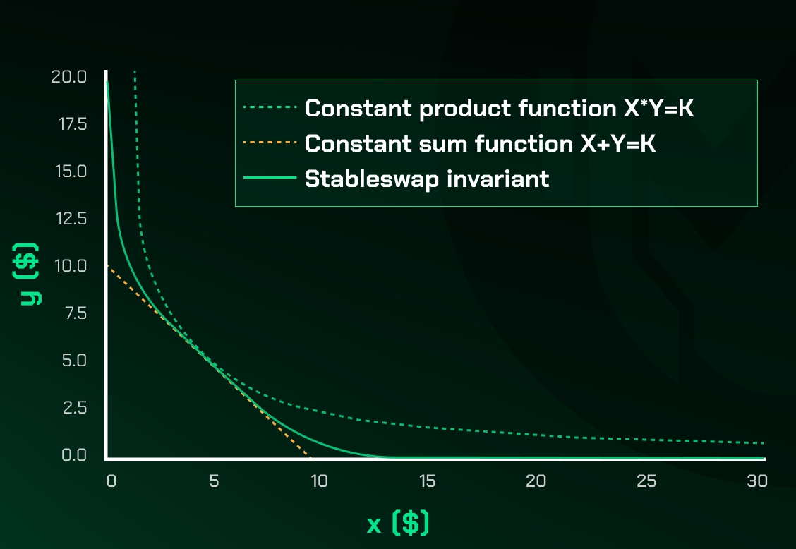
Why stablecoins need special AMMs
Standard constant-product automated market makers (AMMs), like the algorithm behind Uniswap V2, rely on a simple mathematical curve: $x \cdot y = k$. This formula works well for volatile assets where price discovery is the primary goal. However, it is fundamentally inefficient for stablecoins, which are designed to maintain a fixed peg, typically $1.00.
When you trade volatile assets, the price moves significantly with every swap, reflecting market sentiment. With stablecoins, the price should barely move. Under a constant-product model, swapping large amounts of USDC for USDT creates unnecessary slippage. The algorithm treats a $10,000 swap the same as a $100 swap in terms of curve geometry, forcing traders to accept worse rates for large orders. This inefficiency drains liquidity and increases costs for users who simply want to swap one stable asset for another.
StableSwap solves this by combining two mathematical curves into one invariant. It behaves like a constant-sum AMM (linear) when the token prices are close to their peg, allowing for near-zero slippage on large trades. As the price deviates from the peg, it gradually shifts to the constant-product curve (hyperbolic) to protect against depegging risks. This hybrid approach effectively creates a "Uniswap with leverage" for stable assets, offering the deep liquidity of centralized exchanges with the transparency of decentralized protocols.
The chart above shows the USDC/USDT pair. Notice how the price stays tightly bound to the $1.00 line with minimal volatility. This stability is exactly what StableSwap mechanisms are engineered to preserve efficiently, unlike standard AMMs which would show significant price impact on the same volume.
Curve’s StableSwapNG Architecture
Curve Finance has long been the backbone of decentralized stablecoin liquidity, but the original StableSwap contract was built for a simpler era. As DeFi evolved, the need for pools supporting more than two assets became apparent. StableSwapNG is the protocol’s response, designed to handle complex multi-asset swaps without sacrificing the low slippage that defines Curve’s value proposition.
The most significant upgrade in StableSwapNG is the expansion of coin support. While the original Plain Pools were limited to two assets, StableSwapNG allows for up to eight coins in a single pool. This flexibility enables the creation of more efficient liquidity pools for stablecoins that share a common peg, such as USDC, USDT, and DAI, all in one concentrated liquidity layer. Metapools remain capped at two coins, but they can now interact more efficiently with these larger plain pools.
This architectural shift improves capital efficiency by reducing the need for users to split their liquidity across multiple smaller pools. Instead, liquidity is aggregated, which tightens spreads and reduces price impact for traders. The underlying math has been refactored to maintain stability even as the number of assets increases, ensuring that the AMM remains robust against volatility.
| Pool Type | Max Coins | Primary Use Case |
|---|---|---|
| Plain Pool | 8 | Direct swaps between multiple stablecoins |
| Metapool | 2 | Swapping a volatile asset against a stablecoin pool |
| Factory | Variable | Custom pools with specific fee structures |
The codebase for StableSwapNG is open and available on GitHub, allowing developers to deploy permissionless pools that adhere to these new standards. This transparency ensures that the protocol can continue to evolve with the needs of the DeFi ecosystem, providing a scalable solution for stablecoin trading in 2026 and beyond.
PancakeSwap’s implementation approach
PancakeSwap adapted the StableSwap invariant to serve the Binance Smart Chain (BSC) ecosystem, prioritizing speed and low transaction costs alongside capital efficiency. While Curve Finance established the mathematical baseline for stablecoin swaps, PancakeSwap’s implementation focuses on minimizing the friction for users who value BSC’s block time and gas structure. The core mechanism remains identical: a hybrid curve that behaves like a Constant Product Market Maker (CPMM) for large imbalances and like a Constant Sum Market Maker (CSMM) for tight ranges.
The key differentiator lies in the fee structure and liquidity depth distribution. PancakeSwap typically offers lower swap fees on stable pairs compared to standard CPMM pools, incentivizing liquidity providers to keep spreads tight. This directly reduces slippage for traders executing large orders. According to PancakeSwap’s official documentation, the invariant curve is tuned to ensure that small deviations from the peg do not trigger significant price impact, making it ideal for stablecoin arbitrage and hedging.
For BSC users, this means that stable pairs like BUSD/USDT or USDC/DAI can be swapped with minimal slippage even during moderate market volatility. The protocol’s liquidity is often concentrated in these stable pools, creating a deep order book effect without the traditional limit order book infrastructure. This contrasts with Curve’s focus on Ethereum’s higher gas environment, where PancakeSwap’s lower fees provide a competitive edge for high-frequency stablecoin trading.
The result is a trading environment where stablecoins can be swapped with near-zero price impact for most retail-sized transactions. This efficiency is critical for 2026 strategies that rely on rapid capital rotation between stable assets. Traders can enter and exit positions without the slippage penalties that plague standard AMM pools, preserving capital integrity during volatile market conditions.
Osmosis and generalized stableswap
Osmosis has moved beyond the rigid, two-token pools of early DeFi by adopting the Generalized Solidly Stableswap model. This architecture allows for customizable pool parameters, giving liquidity providers and protocol designers granular control over fee structures and swap dynamics. The result is a system that can handle tightly correlated assets across different chains with significantly lower slippage than traditional constant-product models.
The core advantage lies in the flexibility of the invariant function. Unlike older stableswap implementations that locked users into a single fee tier or curve shape, Osmosis allows for multiple fee tiers within the same pool model. This means assets with slightly higher volatility or different utility profiles can still trade efficiently without penalizing stablecoin pairs. The protocol essentially decouples the type of swap (stable vs. volatile) from the cost of the swap, enabling more nuanced liquidity provision strategies.
This customization extends to cross-chain operations. Because Osmosis is built on Cosmos SDK, it leverages IBC (Inter-Blockchain Communication) to facilitate swaps between assets on different chains. The generalized stableswap model ensures that these cross-chain swaps maintain low slippage, provided the assets are tightly correlated. This is particularly useful for bridging stablecoins or wrapped assets between Cosmos chains, where liquidity might be fragmented but the underlying value remains pegged.
To understand how these mechanics perform in practice, we can look at the current market behavior of major stablecoin pairs on the platform. The following chart illustrates the price action and volume dynamics that these generalized pools must navigate.
The ability to customize parameters means that Osmosis can adapt to changing market conditions without requiring hard forks or complex governance proposals for every new asset pair. This adaptability is crucial for maintaining low slippage in a rapidly evolving multi-chain landscape.
LP Yield Strategies in StableSwap Pools
Providing liquidity to StableSwap pools offers a distinct advantage over volatile assets: the near-absence of impermanent loss. Because the assets in these pools remain pegged, the primary risk shifts from price divergence to protocol sustainability and peg stability. For liquidity providers, the goal is to capture trading fees while maintaining exposure to governance incentives.
Fee Accumulation and Trading Volume
The core return for LPs comes from trading fees. StableSwap pools, particularly those on Curve, often see high volume due to their efficiency in swapping pegged assets. Fees are distributed proportionally to LPs based on their share of the pool. Unlike constant-product AMMs where fees might be eaten by slippage, StableSwap’s invariant design ensures that trades execute with minimal price impact, encouraging higher turnover and consistent fee generation.
Governance Voting Power
Many StableSwap protocols, most notably Curve, decouple liquidity provision from governance rights. LPs can lock their LP tokens for a set period (e.g., 4 years) to receive veTokens (vote-escrowed tokens). These veTokens grant voting power over which pools receive gauge rewards. This mechanism allows LPs to direct protocol emissions toward the pools they believe offer the best risk-adjusted returns, effectively creating a secondary layer of yield through boosted incentives.
Managing Peg Risk
While impermanent loss is negligible, peg de-pegging remains the primary risk. If one asset in the pool loses its peg, the StableSwap mechanism will rebalance the pool toward the weaker asset, exposing LPs to significant losses. This is why understanding the underlying assets is critical. LPs should favor pools with strong economic moats and diverse, stable collateral. A de-peg event can wipe out months of fee income in minutes.
Optimizing Yield with veToken Models
To maximize returns, LPs should engage with the governance layer. By locking LP tokens, you not only gain voting power but often receive fee discounts and boosted rewards. This strategy requires a long-term commitment but can significantly amplify yields compared to simply holding LP tokens. The trade-off is liquidity: locked tokens cannot be withdrawn until the lock expires.
No comments yet. Be the first to share your thoughts!